October 19, 2025
In this assignment, a researcher is interested in the effects of drug against stress reaction. She gives a reaction time test to three different groups of subjects: one group that is under a great deal of stress, one group under a moderate amount of stress, and a third group that is under almost no stress. The subjects of the study were instructed to take the drug test during their next stress episode and to report their stress on a scale of 1 to 10 (10 being most pain).
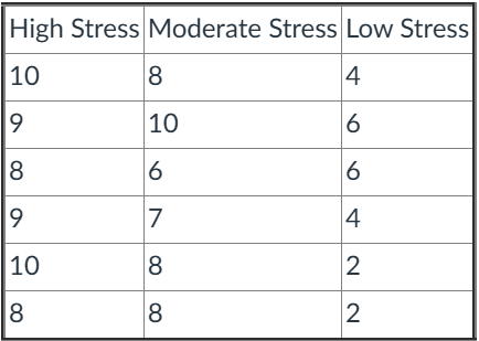
- In R, we can analyze this data using a one-way ANOVA (analysis of variance.) We will start by bringing our data into RStudio. Then creating a data frame composed of values stress and reaction.
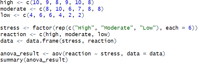
Using these values and data frame, we can conduct use R’s built in function, aov, to analyze and return a summary.
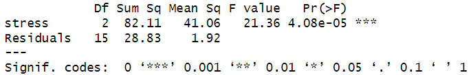
The degrees of freedom (Df) for stress level is 2, representing the number of groups minus one (three stress levels: high, moderate, low → 3 − 1 = 2). The residual degrees of freedom is 15, which is the total number of observations minus the number of groups (18 − 3 = 15).
The Sum of Squares (Sum Sq) indicates how much variability there is in reaction time. The value of 82.11 for “Stress Level” shows how much of the total variation is explained by differences between stress groups. The Residual Sum of Squares (28.83) represents the variation within the groups — that is, how much individuals differ from their own group’s average.
When we divide the Sum of Squares by their respective degrees of freedom, we get the Mean Squares (Mean Sq).
For stress: 82.11 ÷ 2 = 41.06
For residuals: 28.83 ÷ 15 = 1.92
These mean squares are then compared as a ratio to calculate the F value:
F=41.06:1.92=21.36F
The F value (21.36) tells us how much larger the between group variability is compared to the within group variability. In this case, the between group variance is over 21 times greater than the variance within groups — a very strong indication that stress levels have an effect.
Finally, the p-value (Pr(>F)) = 4.08 × 10⁻⁵ is extremely small (well below 0.05). This means there’s less than a 0.005% probability that we’d see such large differences in reaction times by chance if all stress groups were truly equal.
Because the p-value is so small, we reject the null hypothesis. This tells us that stress level has a statistically significant effect on reaction time after taking the drug. In other words, participants under different levels of stress reacted differently — likely with slower responses under higher stress conditions.
2.1 We can see R’s built in dataset zelazo below.
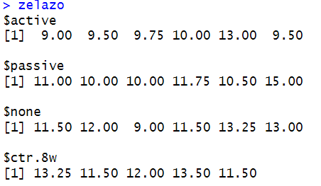
First we need to convert it into a data frame, and then use lm() or aov() to get a summary.
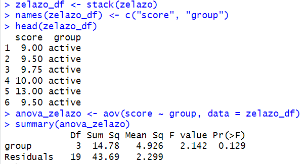
A one way ANOVA was used to compare the effects of four exercise conditions (active, passive, none, and control at 8 weeks) on the age at which infants first started walking. The results showed no significant difference between the groups, F(3, 19) , p = 0.129. This means that the type of exercise did not have a clear effect on walking age, although the active exercise group tended to walk a bit earlier than the others.
To explore this further, the active and passive groups were combined into one exercise group, and the none and control groups were combined into a no-exercise group. A t-test comparing these two combined groups showed that the exercise group walked earlier on average, but the difference was not statistically significant (p > 0.05). Overall, the results suggest that exercise may have a small positive effect on walking age, but there isn’t enough evidence to confirm this with confidence.