October 12, 2024
Regression equation Y = a + bX +e
Where:
Y is the value of the Dependent variable (Y), what is being predicted or explained
a or Alpha, a constant; equals the value of Y when the value of X=0
b or Beta, the coefficient of X; the slope of the regression line; how much Y changes for each one unit change in X.
X is the value of the Independent variable (X), what is predicting or explaining the value of Y
e is the error term; the error in predicting the value of Y, given the value of X (it is not displayed in most regression equations).
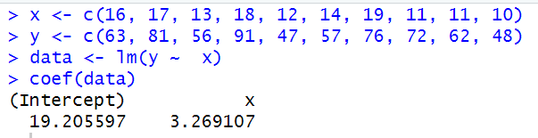
1. Take data set 1:
x <- c(16, 17, 13, 18, 12, 14, 19, 11, 11, 10)
y <- c(63, 81, 56, 91, 47, 57, 76, 72, 62, 48)
1.1 The relationship model between the predictor (x) and the response (y) can be defined as the regression equation. y = a + bx + e
1.2 Using R function lm() and coef() we can calculate the coefficients: a=19.206 and b=3.269, giving us
y = 19.206 + 3.269x
2. Take data set visit:
discharge waiting
1 3.600 79
2 1.800 54
3 3.333 74
4 2.283 62
5 4.533 85
6 2.883 55
If the waiting time since the last eruption has been 80 minutes, to estimate the discharge duration, then waiting would be the predictor or x, and discharge the response variable or y.
We can use the lm() function below to define the relationship model between the predictor and response variable.
lm([target variable] ~ [predictor variables], data = [data source])
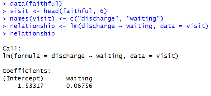
Above, we took dataset visit from dataset faithful, and changed the column names to ‘discharge’ and ‘waiting.’ Then used the lm() function to determine coefficients. Using these, we can determine the relationship:
2.1 discharge = a + b ⋅ waiting + e
2.2 y= -1.533 + 0.068x
(again, with y=discharge, x=waiting time)
2.3 discharge = -1.533 + 0.068(80) = 3.907
The predicted discharge duration if the waiting time since last eruption was 80 minutes is about 3.9 minutes.
3 Displayed below is R’s built in dataset mtcars columns ‘mpg’, ‘disp’, ‘hp’, and ‘wt’.
Again, using lm() allows us to examine the relationship and coefficients of the 4 different variables.
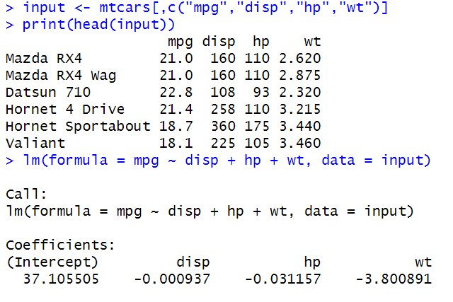
Using the mtcars dataset, the multiple linear regression model predicting miles per gallon (mpg) is:
mpg = 37.11 − (0.00094*disp) − (0.03116*hp) − (3.80×wt)
This means that the baseline mpg is 37.11 when displacement, horsepower, and weight are zero (the intercept). Each unit increase in displacement decreases mpg by 0.00094, each additional horsepower reduces mpg by 0.03116, and each extra 1000 lbs of weight lowers mpg by 3.80, holding other variables constant. Weight has the strongest negative effect on fuel efficiency among the three predictors.
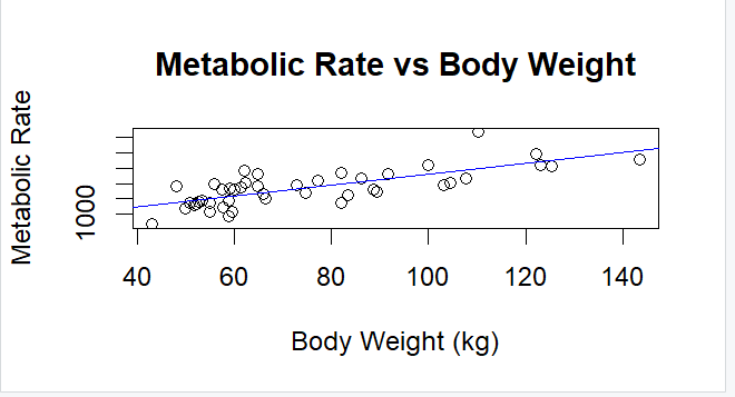
4 pp. 124, 6.5-Exercises # 6.1
Using the rmr data set from the ISwR package in R, we plotted metabolic rate against body weight and fitted a linear regression model to describe their relationship. The plot shows a positive linear trend, and the fitted model confirms that metabolic rate increases with body weight. Based on the regression equation, the predicted metabolic rate for an individual weighing 70 kg is approximately 1300. This prediction is obtained by plugging 70 kg into the fitted linear model.