september 21, 2025
A. Probability
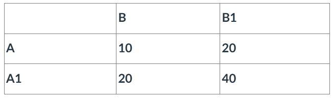
Based on the table below, the probability of:
A1. Event A is 0.333
A2. Event B is 0.333
A3. Event A or B is 0.555
A4. P(A or B) ≠ P(A) + P(B), P(A or B) = P(A) + P(B) – P(A and B)
B. Applying Bayes’ Theorem
Jane is getting married tomorrow, at an outdoor ceremony in the desert. In recent years, it has rained only 5 days each year. Unfortunately, the weatherman has predicted rain for tomorrow. When it actually rains, the weatherman correctly forecasts rain 90% of the time. When it doesn’t rain, he incorrectly forecasts rain 10% of the time.
The sample space is defined by two mutually exclusive events – it rains or it does not rain. Additionally, a third event occurs when the weatherman predicts rain. Notation for these events appears below.
Event A1 – It rains on Jane’s wedding.
Event A2 – It does not rain on Jane’s wedding.
Event B – The weatherman predicts rain.
In terms of probabilities, we know the following:
P(A1) = 5/365 =0.0136985 [It rains 5 days out of the year.]
P(A2) = 360/365 = 0.9863014 [It does not rain 360 days out of the year.]
P(B | A1) = 0.9 [When it rains, the weatherman predicts rain 90% of the time.]
P(B | A2) = 0.1 [When it does not rain, the weatherman predicts rain 10% of the time.]
What is the probability that it will rain on the day of Jane’s wedding?
We want to know P(A1 | B), the probability it will rain on the day of Jane’s wedding, given a forecast for rain by the weatherman. The answer can be determined from Bayes’ theorem, as shown below.
P(A1 | B) = [P(B | A1) * P(A1)] / P(A1) * P(B | A1) + P(A2) * P(B | A2)
P(A1 | B) = (0.9)(0.0136985) / (0.0136985)(0.9) + (0.9863014 )(0.1)
P(A1 | B) = 0.01232865 / 0.11095879
P(A1 | B) = 0.111
The probability that it will rain on the day of Jane’s wedding is 11%.
B1. The original answer is true, the chance of rain, given the forecast, is 11%.
B2. Even though the weatherman correctly predicts rain 90% of the time when it actually rains, the overall chance of rain is low because rain itself is rare. This is an example of the base rate fallacy, where people tend to overlook how uncommon an event is, and focus too much on the accuracy of the prediction. Because most days are dry, even a relatively accurate forecast can still be wrong most of the time when predicting rare events like rain.
C. page 55, #2.3
For a disease known to have a postoperative complication frequency of 20%, a surgeon suggests a new procedure. They test it on 10 patients and found there are not complications. What is the probability of operating on 10 patients successfully with the traditional method?
We can use R’s built in dbinom() function, which can calculate density, distribution function, quantile function, and random generation for the binomial distribution with parameters size and prob.This is conventionally interpreted as the number of ‘successes’ in size trials. In this case, a ‘success’ is a surgery with no complications, which occurs 80% of the time. The sample size is 10 patients, and we are testing to find the probability of success on all 10 patients.
Usage of dbinom() is : dbinom(x, size, prob, log = FALSE)
Input and output into R is shown below.
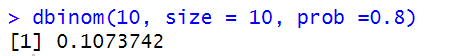
This tells us the probability of having 10 surgeries with 0 complications is 10.73742%.