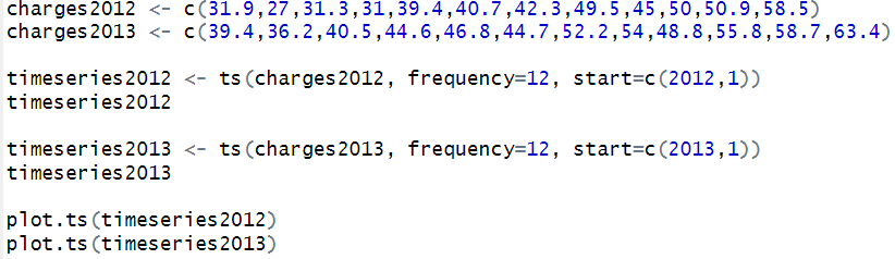
a. This week, we are given a table of data representing charges for a student credit card, and are asked to first construct a time series plot using R.
Using the following code, we are able to plot the charges to the card in 2012 and in 2013.
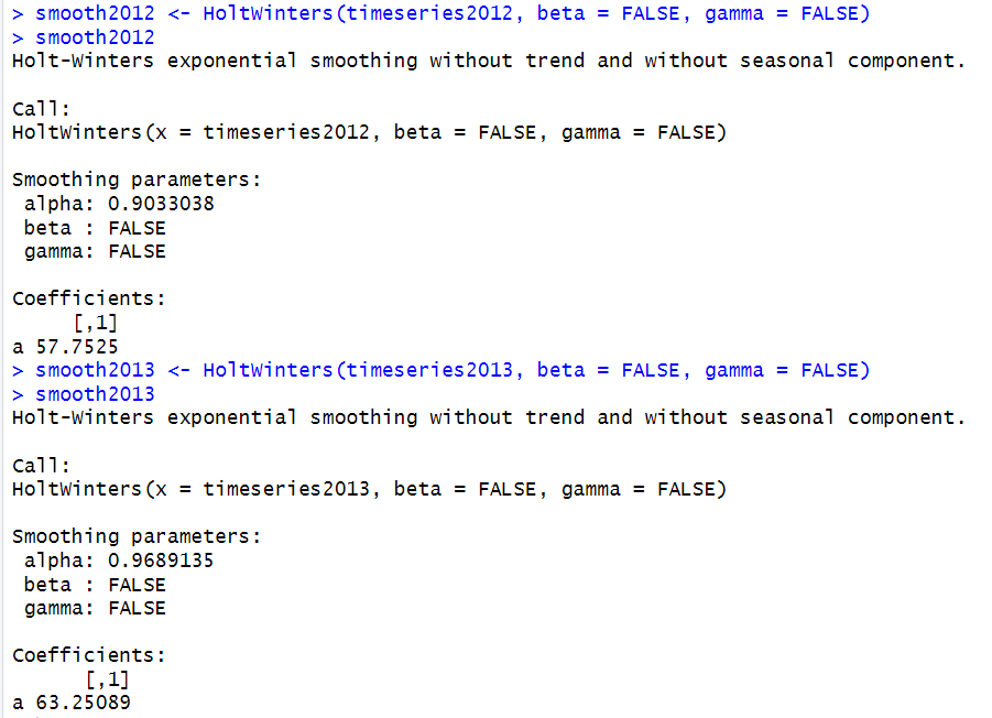
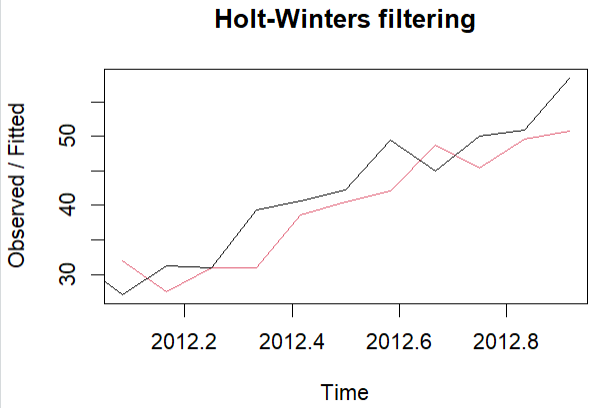
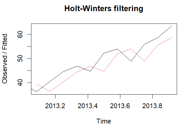
b. Using the HoltWinters() function, we can employ an Exponential Smoothing Model as outlined in Avril Voghlan.‘s notes.
c. The exponential smoothing results show that the smoothing constants (α) for both 2012 and 2013 are very high, at 0.90 and 0.97. This indicates that the model places much greater emphasis on the most recent monthly data, while older observations have less influence on the smoothed estimates.
The final level estimates, $57.75 for 2012 and $63.25 for 2013, represent the average smoothed level of credit card charges at the end of each year. These values reveal that student spending levels rose from 2012 to 2013.
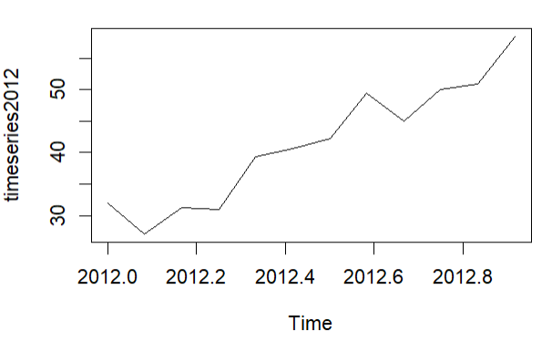
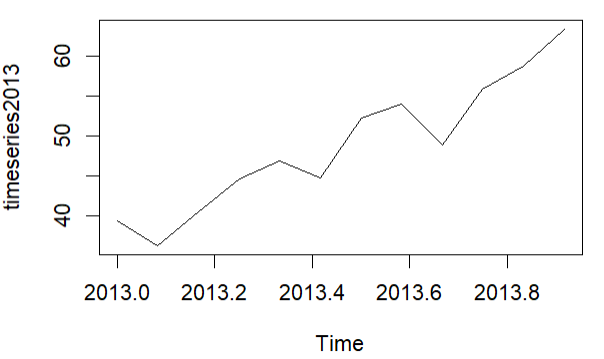
The time series patterns for both years show a steady increase in monthly student credit card charges, peaking in December. This trend suggests that spending rises gradually throughout the year, which could be due to academic and living expenses and seasonal costs such as holiday purchases.